【论文笔记】Instance-Adaptive and Geometric-Aware Keypoint Learning for Category-Level 6D Object Pose Estimation

发表于 2025-02-19 更新于 2025-02-21 分类于读万卷书阅读次数： Waline：本文字数： 5.7k 阅读时长 ≈ 21 分钟

Category-level 6D object pose estimation aims to estimate the rotation, translation and size of unseen instances within specific categories. In this area, dense correspondence-based methods have achieved leading performance. However, they do not explicitly consider the local and global geometric information of different instances, resulting in poor generalization ability to unseen instances with significant shape variations. To deal with this problem, we propose a novel Instance-Adaptive and GeometricAware Keypoint Learning method for category-level 6D object pose estimation (AG-Pose), which includes two key designs: (1) The first design is an Instance-Adaptive Keypoint Detection module, which can adaptively detect a set of sparse keypoints for various instances to represent their geometric structures. (2) The second design is a GeometricAware Feature Aggregation module, which can efficiently integrate the local and global geometric information into keypoint features. These two modules can work together to establish robust keypoint-level correspondences for unseen instances, thus enhancing the generalization ability of the model.Experimental results on CAMERA25 and REAL275 datasets show that the proposed AG-Pose outperforms state-of-the-art methods by a large margin without category-specific shape priors. Code will be released at https://github.com/Leeiieeo/AG-Pose.

Instance-Adaptive and Geometric-Aware Keypoint Learning for Category-Level 6D Object Pose Estimation

方法	类型	训练输入	推理输入	输出	pipeline
AG-Pose	类别级	RGBD + 物体类别	RGBD + 物体类别	绝对\(\mathbf{R}, \mathbf{t}, \mathbf{s}\)

2025.02.19：给我的感觉是一个纯粹的网络方法，没有涉及到什么数学的东西，但是在类别级效果很好

Abstract

1. Introduction

Figure 1. a) The visualization for the correspondence error map and final pose estimation of the dense correspondence-based method, DPDN [17]. Green/red indicates small/large errors and GT/predicted bounding box. b) Points belonging to different parts of the same instance may exhibit similar visual features. Thus, the local geometric information is essential to distinguish them from each other. c) Points belonging to different instances may exhibit similar local geometric structures. Therefore, the global geometric information is crucial for correctly mapping them to the corresponding NOCS coordinates.

In summary, our contributions are as follows:

We propose a novel instance-adaptive and geometricaware keypoint learning method for category-level 6D object pose estimation, which can better generalize to unseen instances with large shape variations. To the best of our knowledge, this is the first adaptive keypoint-based method for category-level 6D object pose estimation.
We evaluate our framework on widely adopted CAMERA25 and REAL275 datasets, and results demonstrate that the proposed method sets a new state-of-the-art performance without using categorical shape priors.

2.1. Instance-level 6D object pose estimation

2.2. Category-level 6D object pose estimation

3. Methodology

Figure 2. a) Overview of the proposed AG-Pose. b) Illustration of the IAKD module. We initialize a set of category-shared learnable queries and convert them into instance-adaptive detectors by integrating the object features. The instance-adaptive detectors are then used to detect keypoints for the object. To guide the learning of the IAKD module, we futher design the L_{div} and L_{ocd} to constrain the distribution of keypoints. c) Illustration of the GAFA module. Our GAFA can efficiently integrate the geometric information into keypoint features through a two-stage feature aggregation process. — Figure 2. a) Overview of the proposed AG-Pose. b) Illustration of the IAKD module. We initialize a set of category-shared learnable queries and convert them into instance-adaptive detectors by integrating the object features. The instance-adaptive detectors are then used to detect keypoints for the object. To guide the learning of the IAKD module, we futher design the \(L_{div}\) and \(L_{ocd}\) to constrain the distribution of keypoints. c) Illustration of the GAFA module. Our GAFA can efficiently integrate the geometric information into keypoint features through a two-stage feature aggregation process.

3.1. Overview

输入RGB-D，先使用MaskRCNN语义分割，得到分割后的RGB图\(\mathbf{I}_{obj} \in \mathbb{R}^{H \times W \times 3}\)和点云\(\mathbf{P}_{obj} \in \mathbb{R}^{N \times 3}\)（\(N\)为点云中点的数量）。

\(\mathbf{P}_{obj}\)会根据相机内参进行反向投影。

以\(\mathbf{I}_{obj}\)和\(\mathbf{P}_{obj}\)为输入，得到\(\mathbf{R} \in SO(3)\)、\(\mathbf{t} \in \mathbb{R}^3\)、\(\mathbf{s} \in \mathbb{R}\)。

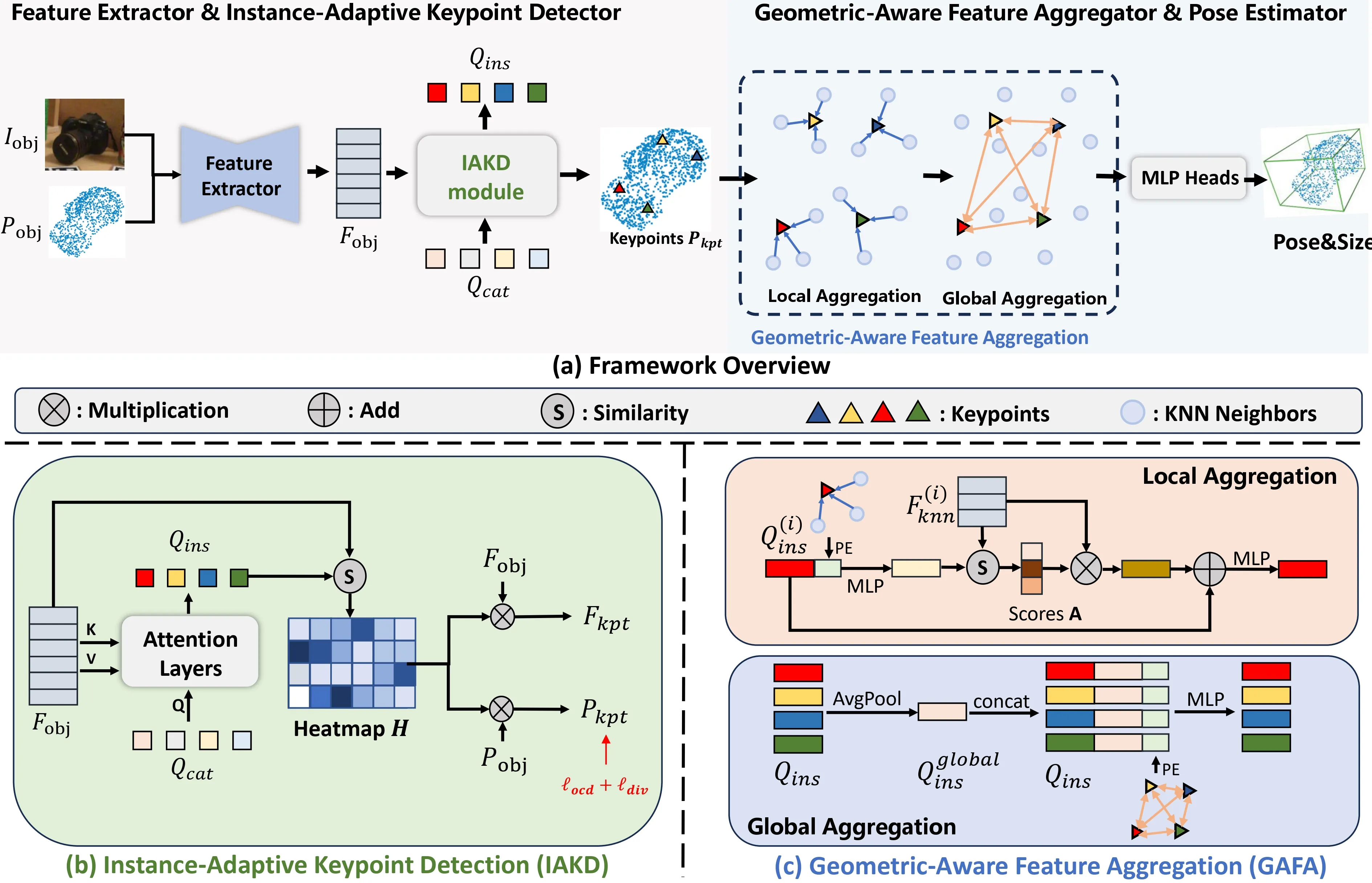
AG-Pose模型框架如图2(a)所示。

3.2. Feature Extractor

对于\(\mathbf{P}_{obj}\)，使用PointNet++从\(\mathbf{P}_{obj}\)中提取特征，得到\(\mathbf{F}_P \in \mathbb{R}^{N \times C_1}\)；
对于\(\mathbf{I}_{obj}\)，遵循“DenseFusion: 6D Object Pose Estimation by Iterative Dense Fusion”，使用PSP Network with ResNet-18提取特征，得到\(\mathbf{F}_I \in \mathbb{R}^{N \times C_2}\)；
将\(\mathbf{F}_P\)和\(\mathbf{F}_I\)进行concat，得到\(\mathbf{F}_{obj} \in \mathbb{R}^{N \times C}\)。

3.3. Instance-Adaptive Keypoint Detector

Figure 3. Illustration of the outlier filter process.

目标是使用稀疏关键点来表示不同实例的形状；
但是问题是推理过程中无法得到实例模型；
所以有了IAKD，以实现检测具有不同形状的实例的关键点。

IAKD模块架构如图2(b)所示。

初始化了类别共享的可学习查询\(\mathbf{Q}_{cat} \in \mathbb{R}^{N_{kpt} \times C}\)，每一个都代表了一个关键点检测器；
使用交叉注意力让\(\mathbf{Q}_{cat}\)作为Q，\(\mathbf{F}_{obj}\)作为K和V，得到\(\mathbf{Q}_{ins} \in \mathbb{R}^{N_{kpt} \times C}\)；
计算\(\mathbf{Q}_{ins}\)和\(\mathbf{F}_{obj}\)的余弦相似度，得到\(\mathbf{H} \in \mathbb{R}^{N_{kpt} \times N}\)；
接下来开始选点选特征，将\(\mathbf{H}\)分别与\(\mathbf{P}_{obj}\)和\(\mathbf{F}_{obj}\)进行相乘，得到\(\mathbf{P}_{kpt} \in \mathbb{R}^{N_{kpt} \times 3}\)和\(\mathbf{F}_{kpt} \in \mathbb{R}^{N_{kpt} \times C}\)。

训练过程中发现关键点往往很聚集，且经常集中分布在非表面或异常值点上。

为了解决关键点聚集问题，设计了损失函数\(L_{div}\)：

\[ L_{div} = \sum_{i = 1}^{N_{kpt}} \sum_{j = 1, j \neq i}^{N_{kpt}} \mathbf{d}(\mathbf{P}_{kpt}^{(i)}, \mathbf{P}_{kpt}^{(j)}), \]

其中：

\[ \mathbf{d}(\mathbf{P}_{kpt}^{(i)}, \mathbf{P}_{kpt}^{(j)}) = \max\left\{th_1 - \Vert \mathbf{P}_{kpt}^{(i)} - \mathbf{P}_{kpt}^{(j)} \Vert_2, 0\right\}, \]

其中，\(th_1\)是一个超参数，\(\mathbf{P}_{kpt}^{(i)}\)代表第\(i\)个关键点；
为了解决关键点集中分布在非表面或异常值点上的问题，首先用\(\mathbf{R}_{gt}\)、\(\mathbf{t}_{gt}\)和\(\mathbf{s}_{gt}\)将\(\mathbf{P}_{obj}\)转换到NOCS空间中，然后使用实例模型\(\mathrm{M}_{obj} \in \mathbb{R}^{M \times 3}\)去除异常值点，得到\(\mathbf{P}_{obj}^\star\)，最后设计了损失函数\(L_{ocd}\)：

\[ \mathbf{P}_{obj}^\star = \left\{x_i|x_i \in \mathbf{P}_{obj} \text{ and } \min_{y_j \in \mathrm{M}_{obj}} \Vert \frac{1}{\Vert \mathbf{s}_{gt} \Vert_2}\mathbf{R}_{gt}(x_i - \mathbf{t}_{gt}) - y_j \Vert_2 < th_2\right\}, \]

其中，\(th_2\)是一个超参数；

最后，\(L_{ocd}\)计算如下：

\[ L_{ocd} = \frac{1}{|\mathbf{P}_{kpt}|} \sum_{x_i \in \mathbf{P}_{kpt}} \min_{y_j \in \mathbf{P}_{obj}^\star} \Vert x_i - y_j \Vert_2. \]

通过将关键点限制为接近\(\mathbf{P}_{obj}^\star\)，IAKD模块可以在推理过程中自动学习过滤掉异常值点。

3.4. Geometric-Aware Feature Aggregator

使用IAKD检测到关键点后，可以直接预测这些关键点在NOCS空间中的坐标，但是这样会缺少几何信息，所以有了GAFA模块。

GAFA模块架构如图2(c)所示。

对于每个关键点，首先在\(\mathbf{P}_{obj}\)中选出\(K\)个邻居和这\(K\)个邻居在\(\mathbf{F}_{obj}\)中对应的特征，得到\(\mathbf{P}_{knn} \in \mathbb{R}^{N_{kpt} \times K \times 3}\)和\(\mathbf{F}_{knn} \in \mathbb{R}^{N_{kpt} \times K \times C}\)；
表示全局几何信息和局部几何信息：
- 全局几何信息可以使用关键点之间的相对位置来表示；
- 局部几何信息可以使用关键点与其相邻点之间的相对位置来表示；
- 分别使用\(\alpha\)和\(\beta\)来表示局部几何信息\(f_l\)和全局几何信息\(f_g\)：
  
  \[ \alpha_{i, j} = MLP(\mathbf{P}_{kpt}^{(i)} - \mathbf{P}_{knn}^{(i, j)}), f_l^{(i)} = AvgPool(\alpha_{i, :}), \]
  
  \[ \beta_{i, j} = MLP(\mathbf{P}_{kpt}^{(i)} - \mathbf{P}_{kpt}^{(j)}), f_g^{(i)} = AvgPool(\beta_{i, :}), \]
  
  其中，\(f_l^{(i)}, f_g^{(i)} \in \mathbb{R}^{1 \times C}\)，\(\mathbf{P}_{knn}^{(i, j)}\)是\(\mathbf{P}_{kpt}^{(i)}\)的第\(j\)个邻居；
将关键点特征\(\mathbf{Q}_{ins}\)与\(f_l\)结合，计算关键点与相邻点之间的局部相关得分\(\mathbf{A}\)，用于聚合来自相邻点的特征，第\(i\)个关键点特征\(\mathbf{Q}_{ins}^{(i)}\)的局部特征聚合过程如下：

\[ \mathbf{A} = sim\left(MLP\left(cat\left[\mathbf{Q}_{ins}^{(i)}, f_l^{(i)}\right]\right), \mathbf{F}_{knn}^{(i)}\right), \]

\[ \mathbf{Q}_{ins}^{(i)} = MLP\left(softmax(\mathbf{A}) \times \mathbf{F}_{knn}^{(i)} + \mathbf{Q}_{ins}^{(i)}\right), \]

上述操作并行执行，以提取具有代表性的局部几何特征；
还需要将全局几何特征\(f_g\)与关键点特征\(\mathbf{Q}_{ins}\)结合：

\[ \mathbf{Q}_{ins}^{global} = AvgPool(\mathbf{Q}_{ins}), \]

\[ \mathbf{Q}_{ins}^{(i)} = MLP\left(concat\left[\mathbf{Q}_{ins}^{(i)}, \mathbf{Q}_{ins}^{global}, f_g^{(i)}\right]\right), \]

其中，\(\mathbf{Q}_{ins}^{global} \in \mathbb{R}^{1 \times C}\)是\(\mathbf{Q}_{ins}\)的全局特征；
上述两阶段聚合允许关键点自适应地聚合来自相邻点的局部几何特征和来自其他关键点的全局几何信息。

3.5. Pose&Size Estimator

然后使用MLP从\(\mathbf{Q}_{ins}\)中预测NOCS坐标点\(\mathbf{P}_{kpt}^{nocs} \in \mathbb{R}^{N_{kpt} \times 3}\)，并通过关键点对应来回归最终的位姿和大小\(\mathbf{R}, \mathbf{t}, \mathbf{s}\)：

\[ \mathbf{P}_{kpt}^{nocs} = MLP(\mathbf{Q}_{ins}), \]

\[ \mathbf{f}_{pose} = concat\left[\mathbf{P}_{kpt}, \mathbf{F}_{kpt}, \mathbf{P}_{kpt}^{nocs}, \mathbf{Q}_{ins}\right], \]

\[ \mathbf{R}, \mathbf{t}, \mathbf{s} = MLP_R(\mathbf{f}_{pose}), MLP_t(\mathbf{f}_{pose}), MLP_s(\mathbf{f}_{pose}). \]

3.6. Overall Loss Function

总的损失函数为：

\[ L_{all} = \lambda_1 L_{ocd} + \lambda_2 L_{div} + \lambda_3 L_{nocs} + \lambda_4 L_{pose}, \]

其中，\(\lambda_1, \lambda_2, \lambda_3, \lambda_4\)为超参数，对于\(L_{pose}\)，这里使用\(L_1\)损失：

\[ L_{pose} = \Vert\mathbf{R}_{gt} - \mathbf{R}\Vert_2 + \Vert\mathbf{t}_{gt} - \mathbf{t}\Vert_2 + \Vert\mathbf{s}_{gt} - \mathbf{s}\Vert_2. \]

使用\(\mathbf{R}_{gt}, \mathbf{t}_{gt}, \mathbf{s}_{gt}\)将相机坐标系下的\(\mathbf{P}_{kpt}\)转换到NOCS空间中，得到关键点的GT NOCS坐标\(\mathbf{P}_{kpt}^{gt}\)，然后使用\(SmoothL_1\)损失：

\[ \mathbf{P}_{kpt}^{gt} = \frac{1}{\Vert \mathbf{s}_{gt} \Vert_2}\mathbf{R}_{gt}(\mathbf{P}_{kpt} - \mathbf{t}_{gt}), \]

\[ L_{nocs} = SmoothL_1(\mathbf{P}_{kpt}^{gt}, \mathbf{P}_{kpt}^{nocs}). \]

4. Experiments

4.1. Comparison with State-of-the-Art Methods

Table 1. Quantitative comparisons with state-of-the-art methods on the REAL275 dataset.
Method	Use of Shape Priors	IoU₅₀	IoU₇₅	5° 2 cm	5° 5 cm	10° 2 cm	10° 5 cm
NOCS [33]	✗	78	30.1	7.2	10	13.8	25.2
DualPoseNet [16]	✗	79.8	62.2	29.3	35.9	50	66.8
GPV-Pose [5]	✗	-	64.4	32	42.9	-	73.3
IST-Net [18]	✗	82.5	76.6	47.5	53.4	72.1	80.5
Query6DoF [35]	✗	82.5	76.1	49	58.9	68.7	83
SPD [28]	✓	77.3	53.2	19.3	21.4	43.2	54.1
SGPA [2]	✓	80.1	61.9	35.9	39.6	61.3	70.7
SAR-Net [15]	✓	79.3	62.4	31.6	42.3	50.3	68.3
RBP-Pose [42]	✓	-	67.8	38.2	48.1	63.1	79.2
DPDN [17]	✓	83.4	76	46	50.7	70.4	78.4
AG-Pose	✗	83.7	79.5	54.7	61.7	74.7	83.1

Table 2. Quantitative comparisons with state-of-the-art methods on the CAMERA25 dataset.
Method	Use of Shape Prior	IoU₅₀	IoU₇₅	5° 2 cm	5° 5 cm	10° 2 cm	10° 5 cm
NOCS [33]	✗	83.9	69.5	32.3	40.9	48.2	64.4
DualPoseNet [16]	✗	92.4	86.4	64.7	70.7	77.2	84.7
GPV-Pose [5]	✗	93.4	88.3	72.1	79.1	-	89
Query6DoF [35]	✗	91.9	88.1	78	83.1	83.9	90
SPD [28]	✓	93.2	83.1	54.3	59	73.3	81.5
SGPA [2]	✓	93.2	88.1	70.7	74.5	82.7	88.4
SAR-Net [15]	✓	86.8	79	66.7	70.9	75.3	80.3
RBP-Pose [42]	✓	93.1	89	73.5	79.6	82.1	89.5
AG-Pose	✗	93.8	91.3	77.8	82.8	85.5	91.6

Figure 4. Comparisons of NOCS error distributions.

4.2. Ablation Studies

Table 3. Comparisons between the IAKD and FPS.
Setting	5° 2 cm	5° 5 cm	10° 2 cm	10° 5 cm
FPS	46.2	55.5	67.0	80.2
IAKD	54.7	61.7	74.7	83.1

Table 4. Ablation studies on the number of keypoints.
\(N_{kpt}\)	5° 2 cm	5° 5 cm	10° 2 cm	10° 5 cm
16	47.9	55.1	68.8	79.8
32	48.8	55.7	73.1	82.9
64	51	57.2	72.8	82
96	54.7	61.7	74.7	83.1
128	52.8	59.9	74.3	83.7

Table 5. Ablation studies on the proposed loss functions.
Loss	5° 2 cm	5° 5 cm	10° 2 cm	10° 5 cm
\(L_{div} + L_{ocd}\)	54.7	61.7	74.7	83.1
\(L_{div} + L_{ucd}\)	49.8	57.3	74.4	82.0
\(L_{div}\)	46.4	53	71	81.3
\(L_{ocd}\)	30	36.1	55.0	68.6
None	29.3	35.6	56.4	69.6

Table 6. Ablation study on two-stage feature aggregation.
Setting	5° 2 cm	5° 5 cm	10° 2 cm	10° 5 cm
Full	54.7	61.7	74.7	83.1
w/o GAFA	47.1	55.3	70.2	80.9
w/o Local	49	57.8	71.2	82.2
w/o Global	50.1	55.8	74.5	82.7
w/ vanilla attn	53	61	72.2	82.1

Table 7. Ablation study on proposed GAFA.
	5° 2 cm	5° 5 cm	10° 2 cm	10° 5 cm
K=8	49.9	57.6	73.1	82.5
K=16	54.7	61.7	74.7	83.1
K=24	54.1	61.1	73.7	83.2
K=32	52.7	59.9	73.6	82.8